记录|深度学习100例-卷积神经网络（CNN）天气识别 | 第5天

这篇博客将从构建自己的天气数据集开始，到定义模型，编译模型，训练模型及验证模型。并进行一些升级，以使得模型更好。
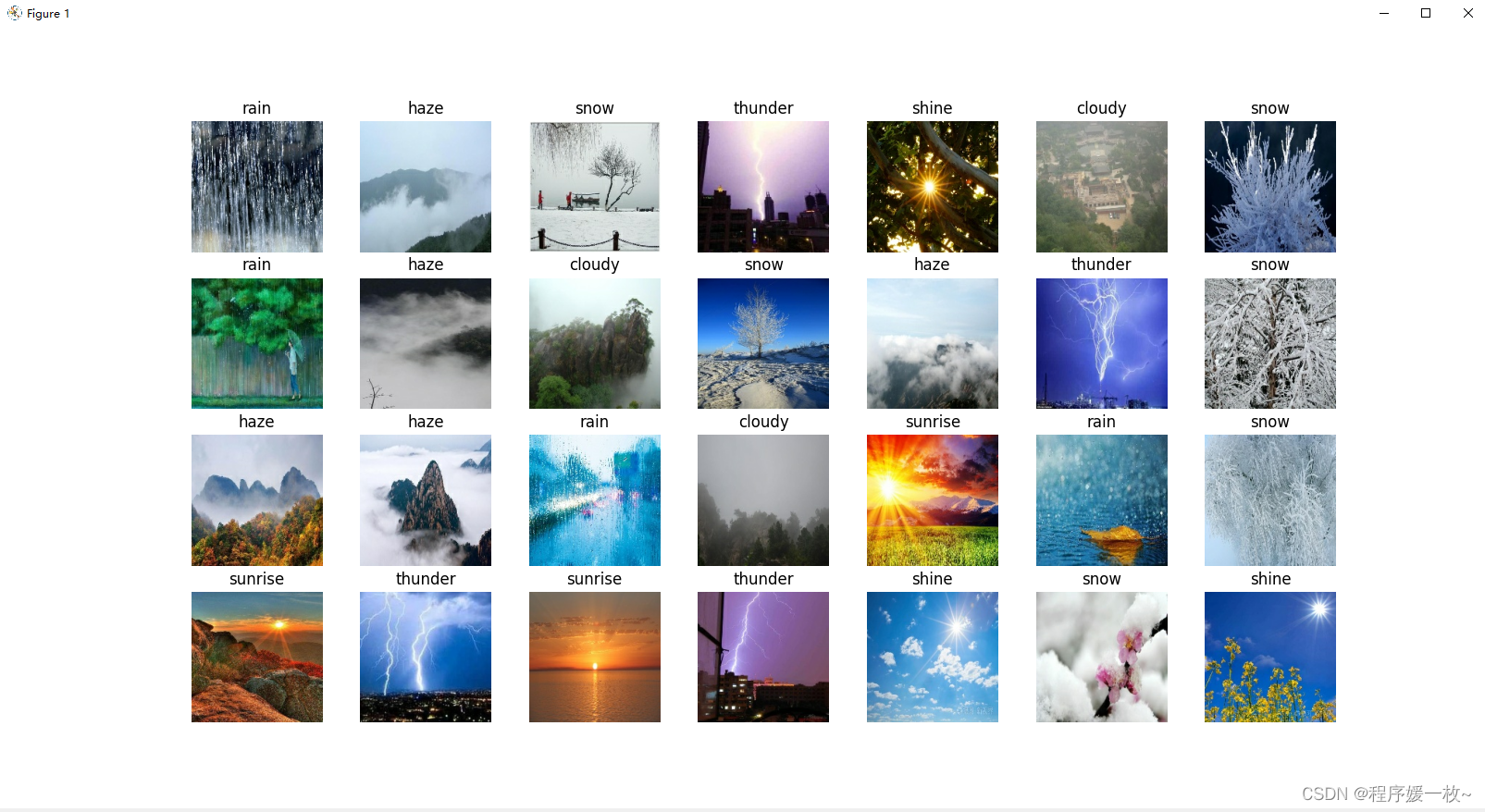
如ImageDateGenerator进行数据增强，之后分别对cloudy，haze，sunrise，shine，snow，rain，thunder等7种天气情况进行识别。

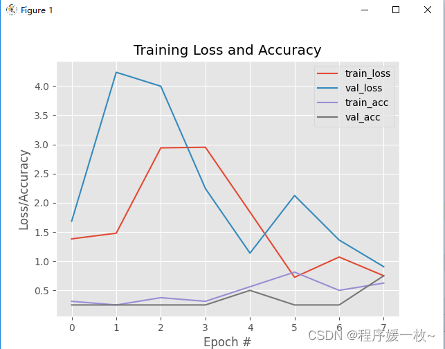
准确率75%不是太高（可能是因为原始数据集的原因，每个分类有4种），可以通过增加原始数据解决。

1. 效果图

原始数据集：

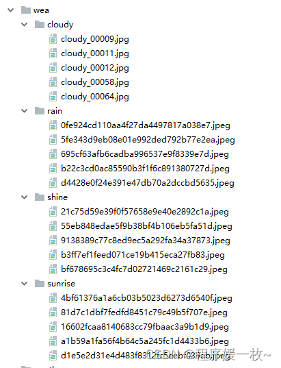
预处理后数据集：（修改了图片名称，调整为固定大小）

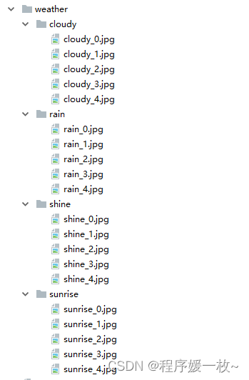
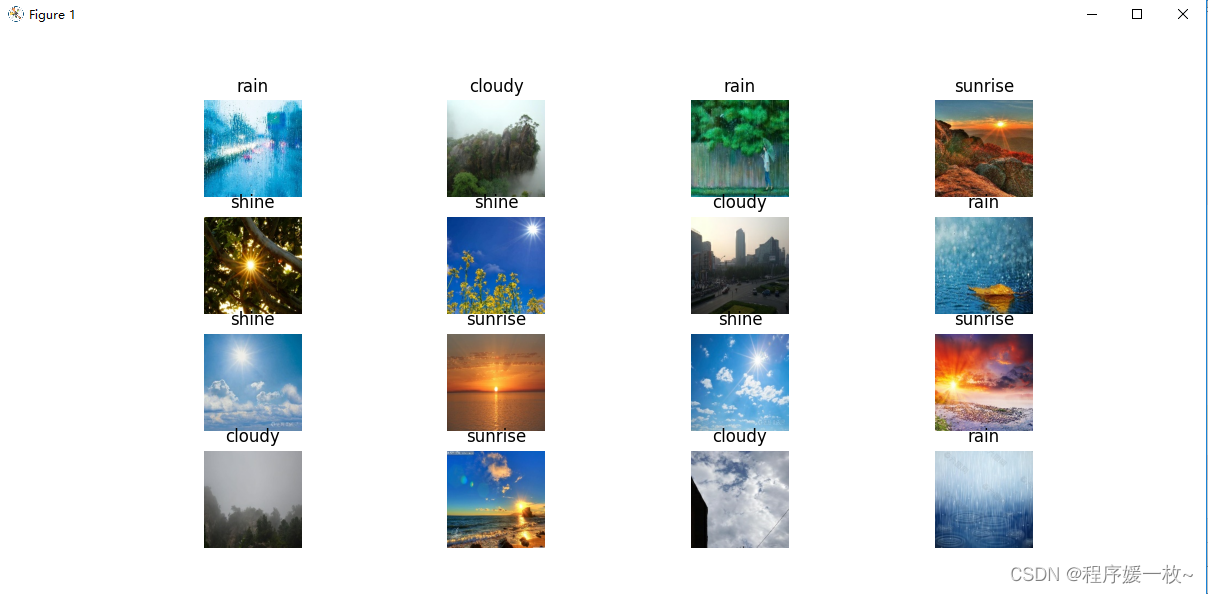
原始训练集图如下：
共20张（rain，cloudy，sunrise，shine各5张），以0.2拆分表示：16张用于训练，4张用于测试。

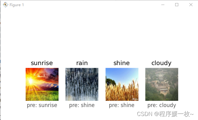
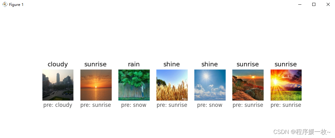
可以看到验证集的图片均成功预测：
title：真实值
pre：预测结果

训练损失/精确度如下：

优化1：数据增强后损失/准确度图：

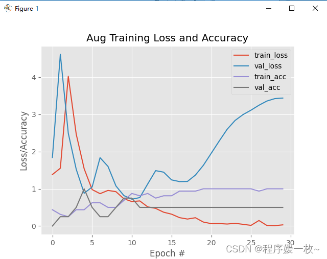
可以看到准确度有提高。

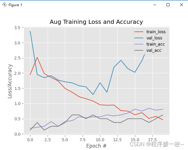
优化2： 数据扩展到并进行数据增强：

2. 源码

2.1 图像预处理源码

# 图像预处理(改名/缩放原图像文件)
# USAGE
# python preprocess_img.pyimport osimport cv2
from imutils import pathsimagePaths = sorted(list(paths.list_images("weather\\")))for num, i in enumerate(imagePaths):src = iprint(num, i)print(str(i.split(os.path.sep)[-2]), str((num + 1) % 5),"weather\\" + str(i.split(os.path.sep)[-2]) + os.path.sep +str(i.split(os.path.sep)[-2]) + "_" + str((num + 1) % 5) + ".jpg")dst = "weather\\" + str(i.split(os.path.sep)[-2]) + os.path.sep + str(i.split(os.path.sep)[-2]) + "_" + str((num + 1) % 5) + ".jpg"# 改名，缩放源文件try:os.rename(src, dst=dst)print('converting %s to %s ...' % (src, dst))except:continueimg = cv2.imread(dst)cv2.imwrite(dst, cv2.resize(img, (180, 180)))

2.2 训练及验证数据源码

# 深度学习100例-卷积神经网络（CNN）天气识别 | 第5天
# usage
# python img_weather5.pyimport pathlibimport matplotlib.pyplot as plt
import numpy as np
import tensorflow as tf
from tensorflow.keras import layers, modelsgpus = tf.config.list_physical_devices("GPU")if gpus:gpu0 = gpus[0]  # 如果有多个GPU，仅使用第0个GPUtf.config.experimental.set_memory_growth(gpu0, True)  # 设置GPU显存用量按需使用tf.config.set_visible_devices([gpu0], "GPU")# 设置随机种子尽可能使结果可以重现
np.random.seed(1)# 设置随机种子尽可能使结果可以重现
tf.random.set_seed(1)# 此处可以为绝对路径/也可以为相对路径
# data_dir = "E:/mat/py-demo-22/220807/weather/"
data_dir = "weather/"# 数据集一共分为cloudy、rain、shine、sunrise
data_dir = pathlib.Path(data_dir)image_count = len(list(data_dir.glob('*/*.jpg')))print("图片总数为：", image_count)batch_size = 32
img_height = 180
img_width = 180"""
关于image_dataset_from_directory()的详细介绍可以参考文章：https://mtyjkh.blog.csdn.net/article/details/117018789
返回的是data = tf.data.Dataset
"""
# 使用image_dataset_from_directory()将数据加载到tf.data.Dataset中
train_ds = tf.keras.preprocessing.image_dataset_from_directory(data_dir,validation_split=0.2,  # 验证集0.2subset="training",seed=123,image_size=(img_height, img_width),batch_size=batch_size)"""
关于image_dataset_from_directory()的详细介绍可以参考文章：https://mtyjkh.blog.csdn.net/article/details/117018789
"""
val_ds = tf.keras.preprocessing.image_dataset_from_directory(data_dir,validation_split=0.2,subset="validation",seed=123,image_size=(img_height, img_width),batch_size=batch_size)class_names = train_ds.class_names
print(class_names)# 可视化
plt.figure(figsize=(16, 8))
for images, labels in train_ds.take(1):for i in range(16):ax = plt.subplot(4, 4, i + 1)# plt.imshow(images[i], cmap=plt.cm.binary)plt.imshow(images[i].numpy().astype("uint8"))plt.title(class_names[labels[i]])plt.axis("off")
plt.show()# 再次检查数据
for image_batch, labels_batch in train_ds:print(image_batch.shape)print(labels_batch.shape)breakAUTOTUNE = tf.data.AUTOTUNE# 将数据集缓存到内存中，加快速度
train_ds = train_ds.cache().shuffle(1000).prefetch(buffer_size=AUTOTUNE)
val_ds = val_ds.cache().prefetch(buffer_size=AUTOTUNE)num_classes = 4"""
关于卷积核的计算不懂的可以参考文章：https://blog.csdn.net/qq_38251616/article/details/114278995
layers.Dropout(0.4) 作用是防止过拟合，提高模型的泛化能力。
在上一篇文章花朵识别中，训练准确率与验证准确率相差巨大就是由于模型过拟合导致的关于Dropout层的更多介绍可以参考文章：https://mtyjkh.blog.csdn.net/article/details/115826689
"""
# 为了增加模型的泛化能力，增加了Dropout层，并将最大池化层更新为平均池化层
model = models.Sequential([layers.experimental.preprocessing.Rescaling(1. / 255, input_shape=(img_height, img_width, 3)),layers.Conv2D(16, (3, 3), activation='relu', input_shape=(img_height, img_width, 3)),  # 卷积层1，卷积核3*3layers.AveragePooling2D((2, 2)),  # 池化层1，2*2采样layers.Conv2D(32, (3, 3), activation='relu'),  # 卷积层2，卷积核3*3layers.AveragePooling2D((2, 2)),  # 池化层2，2*2采样layers.Conv2D(64, (3, 3), activation='relu'),  # 卷积层3，卷积核3*3layers.Dropout(0.3),layers.Flatten(),  # Flatten层，连接卷积层与全连接层layers.Dense(128, activation='relu'),  # 全连接层，特征进一步提取layers.Dense(num_classes)  # 输出层，输出预期结果
])model.summary()  # 打印网络结构# 设置优化器
opt = tf.keras.optimizers.Adam(learning_rate=0.001)model.compile(optimizer=opt,loss=tf.keras.losses.SparseCategoricalCrossentropy(from_logits=True),metrics=['accuracy'])EPOCHS = 8
history = model.fit(train_ds,validation_data=val_ds,epochs=EPOCHS
)for images_test, labels_test in val_ds:continue# 画出训练精确度和损失图
N = np.arange(0, EPOCHS)
plt.style.use("ggplot")
plt.figure()
plt.plot(N, history.history["loss"], label="train_loss")
plt.plot(N, history.history["val_loss"], label="val_loss")
plt.plot(N, history.history["accuracy"], label="train_acc")
plt.plot(N, history.history["val_accuracy"], label="val_acc")
plt.title("Training Loss and Accuracy")
plt.xlabel("Epoch #")
plt.ylabel("Loss/Accuracy")
plt.legend(loc='upper right')  # legend显示位置
plt.show()test_loss, test_acc = model.evaluate(val_ds, verbose=2)
print(test_loss, test_acc)# 优化2 输出在验证集上的预测结果和真实值的对比
pre = model.predict(val_ds)
for images, labels in val_ds.take(1):for i in range(4):ax = plt.subplot(1, 4, i + 1)plt.imshow(images[i].numpy().astype("uint8"))plt.title(class_names[labels[i]])plt.xticks([])plt.yticks([])# plt.xlabel('pre: ' + class_names[np.argmax(pre[i])] + ' real: ' + class_names[labels[i]])plt.xlabel('pre: ' + class_names[np.argmax(pre[i])])print('pre: ' + str(class_names[np.argmax(pre[i])]) + ' real: ' + class_names[labels[i]])
plt.show()print(labels_test)
print(labels)
print(pre)
print(pre.argmax(axis=1))
print(class_names)from sklearn.metrics import classification_report# 优化1 输出可视化报表
print(classification_report(labels_test,pre.argmax(axis=1), target_names=class_names))

2.3 升级版+数据增强训练及验证数据源码

# 深度学习100例-卷积神经网络（CNN）天气识别 | 第5天
# usage
# python img_weather5_aug.pyimport pathlibimport matplotlib.pyplot as plt
import numpy as np
import tensorflow as tf
from tensorflow.keras import layers, models
# 将使用ImageDataGenerator扩充数据。建议使用数据扩充，这样会导致模型更好地推广。
# 数据扩充涉及对现有训练数据添加随机旋转，平移，剪切和缩放比例。
from tensorflow.keras.preprocessing.image import ImageDataGeneratorgpus = tf.config.list_physical_devices("GPU")if gpus:gpu0 = gpus[0]  # 如果有多个GPU，仅使用第0个GPUtf.config.experimental.set_memory_growth(gpu0, True)  # 设置GPU显存用量按需使用tf.config.set_visible_devices([gpu0], "GPU")# 设置随机种子尽可能使结果可以重现
np.random.seed(1)# 设置随机种子尽可能使结果可以重现
tf.random.set_seed(1)# 此处可以为绝对路径/也可以为相对路径
# data_dir = "E:/mat/py-demo-22/220807/weather/"
data_dir = "weather/"# 数据集一共分为cloudy、rain、shine、sunrise
data_dir = pathlib.Path(data_dir)image_count = len(list(data_dir.glob('*/*.jpg')))print("图片总数为：", image_count)batch_size = 32
img_height = 180
img_width = 180"""
关于image_dataset_from_directory()的详细介绍可以参考文章：https://mtyjkh.blog.csdn.net/article/details/117018789
返回的是data = tf.data.Dataset
"""
# 使用image_dataset_from_directory()将数据加载到tf.data.Dataset中
train_ds = tf.keras.preprocessing.image_dataset_from_directory(data_dir,validation_split=0.2,  # 验证集0.2subset="training",seed=123,image_size=(img_height, img_width),batch_size=batch_size)"""
关于image_dataset_from_directory()的详细介绍可以参考文章：https://mtyjkh.blog.csdn.net/article/details/117018789
"""
val_ds = tf.keras.preprocessing.image_dataset_from_directory(data_dir,validation_split=0.2,subset="validation",seed=123,image_size=(img_height, img_width),batch_size=batch_size)class_names = train_ds.class_names
print(class_names)# 可视化
plt.figure(figsize=(16, 8))
for images, labels in train_ds.take(1):for i in range(16):ax = plt.subplot(4, 4, i + 1)# plt.imshow(images[i], cmap=plt.cm.binary)plt.imshow(images[i].numpy().astype("uint8"))plt.title(class_names[labels[i]])plt.axis("off")
plt.show()# 再次检查数据
for image_batch, labels_batch in train_ds:print(image_batch.shape)print(labels_batch.shape)break# 构建图像加强生成器
# 图像增强使我们可以通过随机旋转，移动，剪切，缩放和翻转从现有的训练数据中构建“其他”训练数据。
# 数据扩充通常是以下关键步骤：
# -避免过度拟合
# -确保模型能很好地泛化  我建议您始终执行数据增强，除非您有明确的理由不这样做。
aug = ImageDataGenerator(rotation_range=30, width_shift_range=0.1,height_shift_range=0.1, shear_range=0.2, zoom_range=0.2,horizontal_flip=True, fill_mode="nearest")
x = aug.flow(image_batch, labels_batch)# 可视化
plt.figure(figsize=(16, 8))
for image_batch, labels_batch in x:print(image_batch.shape)print(labels_batch.shape)break
print(x.x.shape)
for i in range(16):ax = plt.subplot(4, 4, i + 1)plt.imshow(x.x[i].astype("uint8"))plt.title(class_names[labels[i]])plt.axis("off")
plt.show()AUTOTUNE = tf.data.AUTOTUNE# 将数据集缓存到内存中，加快速度
train_ds = train_ds.cache().shuffle(1000).prefetch(buffer_size=AUTOTUNE)
val_ds = val_ds.cache().prefetch(buffer_size=AUTOTUNE)num_classes = 4"""
关于卷积核的计算不懂的可以参考文章：https://blog.csdn.net/qq_38251616/article/details/114278995
layers.Dropout(0.4) 作用是防止过拟合，提高模型的泛化能力。
在上一篇文章花朵识别中，训练准确率与验证准确率相差巨大就是由于模型过拟合导致的关于Dropout层的更多介绍可以参考文章：https://mtyjkh.blog.csdn.net/article/details/115826689
"""
# 为了增加模型的泛化能力，增加了Dropout层，并将最大池化层更新为平均池化层
model = models.Sequential([layers.experimental.preprocessing.Rescaling(1. / 255, input_shape=(img_height, img_width, 3)),layers.Conv2D(16, (3, 3), activation='relu', input_shape=(img_height, img_width, 3)),  # 卷积层1，卷积核3*3layers.AveragePooling2D((2, 2)),  # 池化层1，2*2采样layers.Conv2D(32, (3, 3), activation='relu'),  # 卷积层2，卷积核3*3layers.AveragePooling2D((2, 2)),  # 池化层2，2*2采样layers.Conv2D(64, (3, 3), activation='relu'),  # 卷积层3，卷积核3*3layers.Dropout(0.3),layers.Flatten(),  # Flatten层，连接卷积层与全连接层layers.Dense(128, activation='relu'),  # 全连接层，特征进一步提取layers.Dense(num_classes)  # 输出层，输出预期结果
])model.summary()  # 打印网络结构# 设置优化器
opt = tf.keras.optimizers.Adam(learning_rate=0.001)model.compile(optimizer=opt,loss=tf.keras.losses.SparseCategoricalCrossentropy(from_logits=True),metrics=['accuracy'])EPOCHS = 20
BS = 32# 训练网络
# model.fit 可同时处理训练和即时扩充的增强数据。
# 我们必须将训练数据作为第一个参数传递给生成器。生成器将根据我们先前进行的设置生成批量的增强训练数据。
for images_train, labels_train in train_ds:continue
for images_test, labels_test in val_ds:continue
history = model.fit(x=aug.flow(images_train,labels_train, batch_size=BS),validation_data=(images_test, labels_test), steps_per_epoch=1,epochs=EPOCHS)# 画出训练精确度和损失图
N = np.arange(0, EPOCHS)
plt.style.use("ggplot")
plt.figure()
plt.plot(N, history.history["loss"], label="train_loss")
plt.plot(N, history.history["val_loss"], label="val_loss")
plt.plot(N, history.history["accuracy"], label="train_acc")
plt.plot(N, history.history["val_accuracy"], label="val_acc")
plt.title("Aug Training Loss and Accuracy")
plt.xlabel("Epoch #")
plt.ylabel("Loss/Accuracy")
plt.legend(loc='upper right')  # legend显示位置
plt.show()test_loss, test_acc = model.evaluate(val_ds, verbose=2)
print(test_loss, test_acc)# 优化2 输出在验证集上的预测结果和真实值的对比
pre = model.predict(val_ds)
for images, labels in val_ds.take(1):for i in range(4):ax = plt.subplot(1, 4, i + 1)plt.imshow(images[i].numpy().astype("uint8"))plt.title(class_names[labels[i]])plt.xticks([])plt.yticks([])# plt.xlabel('pre: ' + class_names[np.argmax(pre[i])] + ' real: ' + class_names[labels[i]])plt.xlabel('pre: ' + class_names[np.argmax(pre[i])])print('pre: ' + str(class_names[np.argmax(pre[i])]) + ' real: ' + class_names[labels[i]])
plt.show()print(labels_test)
print(labels)
print(pre)
print(class_names)
from sklearn.metrics import classification_report
# 优化1 输出可视化报表
print(classification_report(labels_test,pre.argmax(axis=1), target_names=class_names))

参考

• Keras TensorFlow教程：使用自己的数据集进行训练
• https://mtyjkh.blog.csdn.net/article/details/117186183
• 天气数据集 ~~ 文末下载
• 天气原始数据集处理参考