使用Python，OpenCV对图像进行亚像素点检测，并拟合椭圆进行绘制

这篇博客将介绍如何使用Python，OpenCV对图像进行亚像素检测，并对亚像素点进行椭圆拟合绘制。

1. 效果图

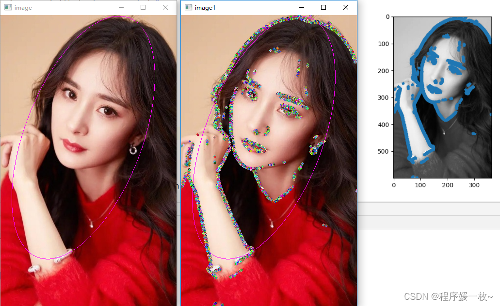
原始图上绘制拟合椭圆 VS 原始图上绘制拟合椭圆及亚像素点绘制随机半径及颜色的圆 VS 灰度图上绘制亚像素点效果图如下：
在这里插入图片描述
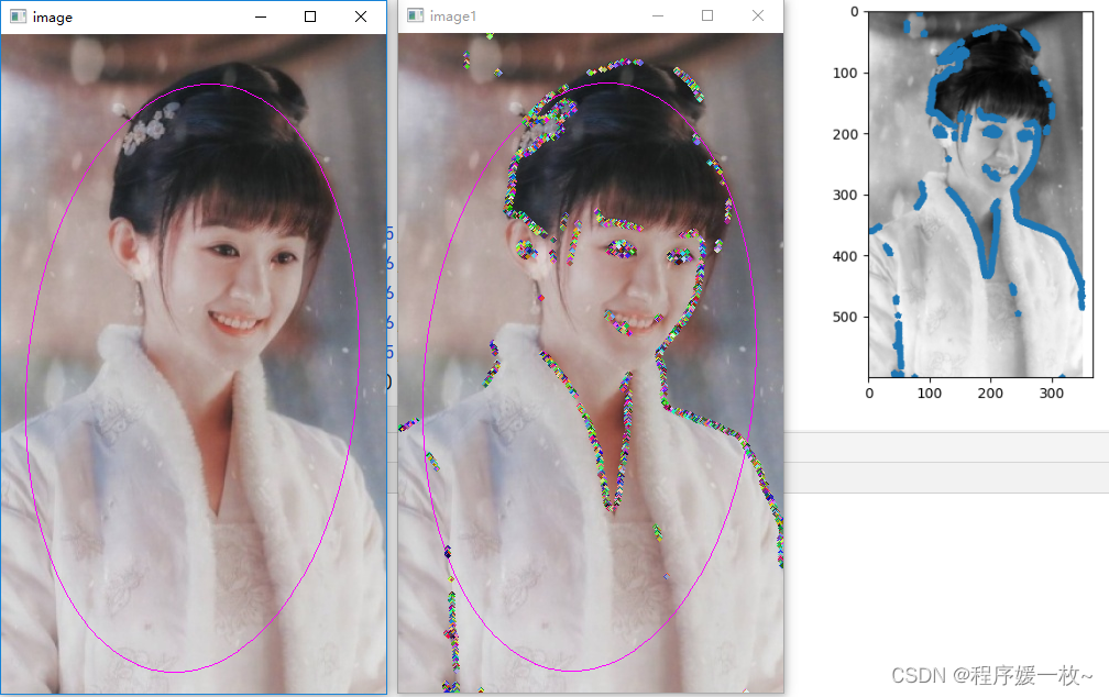
我喜欢的颖宝效果图2如下：

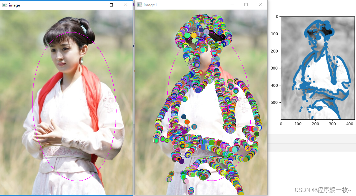
圆的随机半径放大一点效果图如下：

2. 源码

需要注意，绘制圆需要圆心都是int值

# 计算图像的亚像素点并绘制（matplotlib以及cv2），并对亚像素点进行3种椭圆方式拟合绘制
# python zernick_detection.pyimport timeimport cv2
import imutils
import matplotlib.pyplot as plt
import numpy as npg_N = 7M00 = np.array([0, 0.0287, 0.0686, 0.0807, 0.0686, 0.0287, 0,0.0287, 0.0815, 0.0816, 0.0816, 0.0816, 0.0815, 0.0287,0.0686, 0.0816, 0.0816, 0.0816, 0.0816, 0.0816, 0.0686,0.0807, 0.0816, 0.0816, 0.0816, 0.0816, 0.0816, 0.0807,0.0686, 0.0816, 0.0816, 0.0816, 0.0816, 0.0816, 0.0686,0.0287, 0.0815, 0.0816, 0.0816, 0.0816, 0.0815, 0.0287,0, 0.0287, 0.0686, 0.0807, 0.0686, 0.0287, 0]).reshape((7, 7))M11R = np.array([0, -0.015, -0.019, 0, 0.019, 0.015, 0,-0.0224, -0.0466, -0.0233, 0, 0.0233, 0.0466, 0.0224,-0.0573, -0.0466, -0.0233, 0, 0.0233, 0.0466, 0.0573,-0.069, -0.0466, -0.0233, 0, 0.0233, 0.0466, 0.069,-0.0573, -0.0466, -0.0233, 0, 0.0233, 0.0466, 0.0573,-0.0224, -0.0466, -0.0233, 0, 0.0233, 0.0466, 0.0224,0, -0.015, -0.019, 0, 0.019, 0.015, 0]).reshape((7, 7))M11I = np.array([0, -0.0224, -0.0573, -0.069, -0.0573, -0.0224, 0,-0.015, -0.0466, -0.0466, -0.0466, -0.0466, -0.0466, -0.015,-0.019, -0.0233, -0.0233, -0.0233, -0.0233, -0.0233, -0.019,0, 0, 0, 0, 0, 0, 0,0.019, 0.0233, 0.0233, 0.0233, 0.0233, 0.0233, 0.019,0.015, 0.0466, 0.0466, 0.0466, 0.0466, 0.0466, 0.015,0, 0.0224, 0.0573, 0.069, 0.0573, 0.0224, 0]).reshape((7, 7))M20 = np.array([0, 0.0225, 0.0394, 0.0396, 0.0394, 0.0225, 0,0.0225, 0.0271, -0.0128, -0.0261, -0.0128, 0.0271, 0.0225,0.0394, -0.0128, -0.0528, -0.0661, -0.0528, -0.0128, 0.0394,0.0396, -0.0261, -0.0661, -0.0794, -0.0661, -0.0261, 0.0396,0.0394, -0.0128, -0.0528, -0.0661, -0.0528, -0.0128, 0.0394,0.0225, 0.0271, -0.0128, -0.0261, -0.0128, 0.0271, 0.0225,0, 0.0225, 0.0394, 0.0396, 0.0394, 0.0225, 0]).reshape((7, 7))M31R = np.array([0, -0.0103, -0.0073, 0, 0.0073, 0.0103, 0,-0.0153, -0.0018, 0.0162, 0, -0.0162, 0.0018, 0.0153,-0.0223, 0.0324, 0.0333, 0, -0.0333, -0.0324, 0.0223,-0.0190, 0.0438, 0.0390, 0, -0.0390, -0.0438, 0.0190,-0.0223, 0.0324, 0.0333, 0, -0.0333, -0.0324, 0.0223,-0.0153, -0.0018, 0.0162, 0, -0.0162, 0.0018, 0.0153,0, -0.0103, -0.0073, 0, 0.0073, 0.0103, 0]).reshape(7, 7)M31I = np.array([0, -0.0153, -0.0223, -0.019, -0.0223, -0.0153, 0,-0.0103, -0.0018, 0.0324, 0.0438, 0.0324, -0.0018, -0.0103,-0.0073, 0.0162, 0.0333, 0.039, 0.0333, 0.0162, -0.0073,0, 0, 0, 0, 0, 0, 0,0.0073, -0.0162, -0.0333, -0.039, -0.0333, -0.0162, 0.0073,0.0103, 0.0018, -0.0324, -0.0438, -0.0324, 0.0018, 0.0103,0, 0.0153, 0.0223, 0.0190, 0.0223, 0.0153, 0]).reshape(7, 7)M40 = np.array([0, 0.013, 0.0056, -0.0018, 0.0056, 0.013, 0,0.0130, -0.0186, -0.0323, -0.0239, -0.0323, -0.0186, 0.0130,0.0056, -0.0323, 0.0125, 0.0406, 0.0125, -0.0323, 0.0056,-0.0018, -0.0239, 0.0406, 0.0751, 0.0406, -0.0239, -0.0018,0.0056, -0.0323, 0.0125, 0.0406, 0.0125, -0.0323, 0.0056,0.0130, -0.0186, -0.0323, -0.0239, -0.0323, -0.0186, 0.0130,0, 0.013, 0.0056, -0.0018, 0.0056, 0.013, 0]).reshape(7, 7)def zernike_detection(path):img = cv2.imread(path)img = cv2.cvtColor(img, cv2.COLOR_BGR2GRAY)blur_img = cv2.medianBlur(img, 13)c_img = cv2.adaptiveThreshold(blur_img, 255, cv2.ADAPTIVE_THRESH_GAUSSIAN_C, cv2.THRESH_BINARY_INV, 7, 4)ZerImgM00 = cv2.filter2D(c_img, cv2.CV_64F, M00)ZerImgM11R = cv2.filter2D(c_img, cv2.CV_64F, M11R)ZerImgM11I = cv2.filter2D(c_img, cv2.CV_64F, M11I)ZerImgM20 = cv2.filter2D(c_img, cv2.CV_64F, M20)ZerImgM31R = cv2.filter2D(c_img, cv2.CV_64F, M31R)ZerImgM31I = cv2.filter2D(c_img, cv2.CV_64F, M31I)ZerImgM40 = cv2.filter2D(c_img, cv2.CV_64F, M40)point_temporary_x = []point_temporary_y = []scatter_arr = cv2.findNonZero(ZerImgM00).reshape(-1, 2)for idx in scatter_arr:j, i = idxtheta_temporary = np.arctan2(ZerImgM31I[i][j], ZerImgM31R[i][j])rotated_z11 = np.sin(theta_temporary) * ZerImgM11I[i][j] + np.cos(theta_temporary) * ZerImgM11R[i][j]rotated_z31 = np.sin(theta_temporary) * ZerImgM31I[i][j] + np.cos(theta_temporary) * ZerImgM31R[i][j]l_method1 = np.sqrt((5 * ZerImgM40[i][j] + 3 * ZerImgM20[i][j]) / (8 * ZerImgM20[i][j]))l_method2 = np.sqrt((5 * rotated_z31 + rotated_z11) / (6 * rotated_z11))l = (l_method1 + l_method2) / 2k = 3 * rotated_z11 / (2 * (1 - l_method2 ** 2) ** 1.5)# h = (ZerImgM00[i][j] - k * np.pi / 2 + k * np.arcsin(l_method2) + k * l_method2 * (1 - l_method2 ** 2) ** 0.5)# / np.pik_value = 20.0l_value = 2 ** 0.5 / g_Nabsl = np.abs(l_method2 - l_method1)if k >= k_value and absl <= l_value:y = i + g_N * l * np.sin(theta_temporary) / 2x = j + g_N * l * np.cos(theta_temporary) / 2point_temporary_x.append(x)point_temporary_y.append(y)else:continuereturn point_temporary_x, point_temporary_yimage = cv2.imread('ml2.jpg')
path = 'ym_600.jpg'
cv2.imwrite(path, imutils.resize(image, height=600))time1 = time.time()
point_temporary_x, point_temporary_y = zernike_detection(path)
time2 = time.time()
print(time2 - time1)# gray : 进行检测的图像
gray = cv2.imread(path, 0)
plt.imshow(gray, cmap="gray")
# point检测出的亚像素点
point = np.array([point_temporary_x, point_temporary_y])
# s:调整显示点的大小
plt.scatter(point[0, :], point[1, :], s=10, marker="*")
plt.show()def cv_fit_ellipse(points, flag=0):# cv2.fitEllipse only can estimate int numpy 2D array datap = np.array(points)p = np.array(p).astype(int)center0, axes0, angle0 = cv2.fitEllipse(p)center1, axes1, angle1 = cv2.fitEllipseAMS(p)center2, axes2, angle2 = cv2.fitEllipseDirect(p)print(type(center0))print("fitEllipse:       " + str(np.array(center0)))print("fitEllipseAMS:    " + str(np.array(center1)))print("fitEllipseDirect: " + str(np.array(center2)))box = tuple([tuple(np.array(center0)), tuple(np.array(axes0)), angle0])if flag == 0:box = tuple([tuple(np.array(center0)), tuple(np.array(axes0)), angle0])elif flag == 1:box = tuple([tuple(np.array(center1)), tuple(np.array(axes1)), angle1])else:box = tuple([tuple(np.array(center0)), tuple(np.array(axes0)), angle0])return boxpoints = np.array(list(zip(point_temporary_x, point_temporary_y)))
print(type(points), points[0], points.shape)
box1 = cv_fit_ellipse(points, flag=1)image = cv2.imread(path)cv2.ellipse(img=image, box=box1, color=(255, 0, 255), thickness=1)
cv2.imshow("image", image)
for i in points:# 亚像素点绘制随机颜色半径圆radius = np.random.randint(1, high=10)color = np.random.randint(0, high=256, size=(3,)).tolist()# print('radius: ', radius, type(radius))# print('color: ', color, type(color))cv2.circle(image, (int(i[0]), int(i[1])), radius, color, -1)cv2.imshow("image1", image)
cv2.waitKey(0)
cv2.destroyAllWindows()