使用Python，PCA对iris数据集降维2维/3维并进行2D，3D散点图绘制（包括有图例无图例，有标题Label无标题Label）

这篇博客将介绍如何使用Python，PCA对iris数据集降维2，3并进行2D,3D散点图绘制（包括有图例&无图例，有标题Label&无标题Label）。
着重介绍怎么一次性添加多类型的图例到图表，通过显式获取scatter。

# 方法1
scatter = ax.scatter(x_reduced[:, 0], x_reduced[:, 1], x_reduced[:, 2], c=iris.target)
# 方法2
scatter = plt.scatter(x_reduced[:, 0], x_reduced[:, 1], c=iris.target, marker="d")
# 添加图例名称到图标
plt.legend(handles=scatter.legend_elements()[0],labels=sp_names,title="species", loc="upper right")

1. 效果图

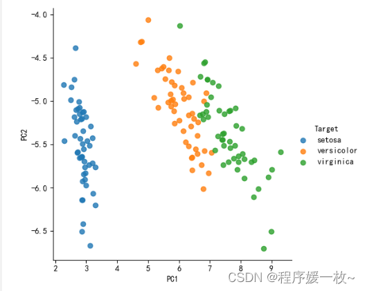
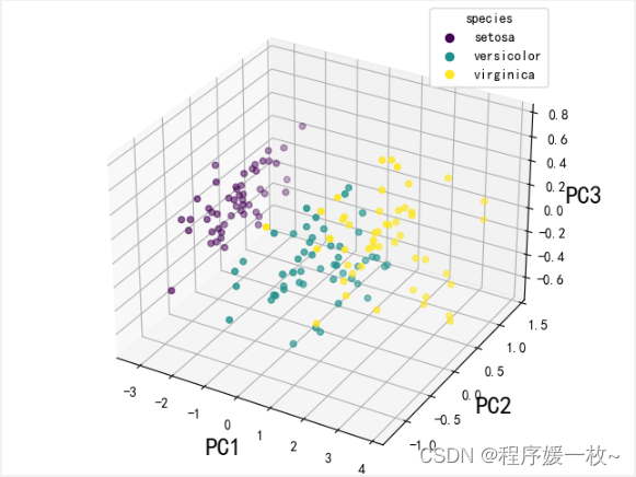
对鸢尾花进行PCA降维成2维后进行绘制，Seaborn效果图如下：
在这里插入图片描述

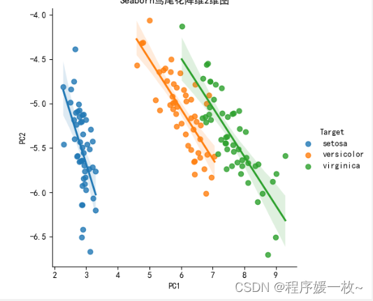
对鸢尾花进行PCA降维成2维后进行绘制，Seaborn添加标题及散点拟合线效果图如下：

在这里插入图片描述

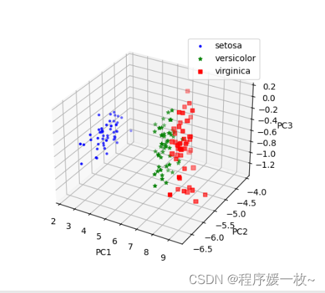
对鸢尾花进行PCA降维成3维后进行绘制，Matplotlib3D效果图如下：

在这里插入图片描述
对鸢尾花进行PCA降维成3维简单绘制效果图如下：

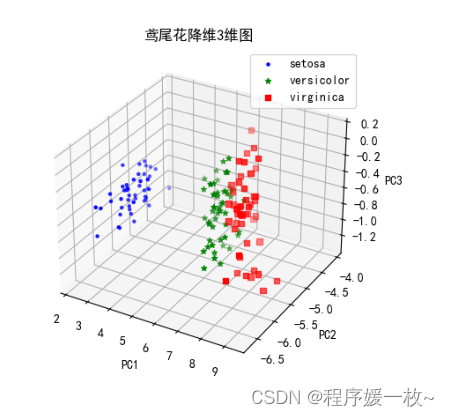
对鸢尾花进行PCA降维成3维后进行绘制，添加中文标题，xyz轴描述及图例，不同类型用不同的样式mark 效果图如下：
在这里插入图片描述

2. 源码

# 使用PCA对鸢尾花特征进行降维2维/3维并绘制 2D,3D散点图（有图例&无图例，有标题Lable&无标题Lable）
# python iris_pca.py
import matplotlib.pyplot as plt
import numpy as np
import pandas as pd
import seaborn as sns
from mpl_toolkits.mplot3d import Axes3D
from sklearn import datasets
from sklearn.decomposition import PCA# 支持中文
plt.rcParams['font.sans-serif'] = ['SimHei']
plt.rcParams['axes.unicode_minus'] = Falseiris = datasets.load_iris()
R = np.array(iris.data)R_cov = np.cov(R, rowvar=False)iris_covmat = pd.DataFrame(data=R_cov, columns=iris.feature_names)
iris_covmat.index = iris.feature_names
eig_values, eig_vectors = np.linalg.eig(R_cov)def plot_2D_Seaborn():featureVector = eig_vectors[:, :2]featureVector_t = np.transpose(featureVector)# R is the original iris datasetR_t = np.transpose(R)newDataset_t = np.matmul(featureVector_t, R_t)newDataset = np.transpose(newDataset_t)# 可视化 绘制2D图# 鸢尾花数据创建dataframedf = pd.DataFrame(data=newDataset, columns=['PC1', 'PC2'])y = pd.Series(iris.target)y = y.replace(0, 'setosa')y = y.replace(1, 'versicolor')y = y.replace(2, 'virginica')df['Target'] = y# 绘制2维数据，fit_reg是否拟合线sns.lmplot(x='PC1', y='PC2', data=df, hue='Target', fit_reg=False, legend=True)# sns.lmplot(x='PC1', y='PC2', data=df, hue='Target', fit_reg=True, legend=True)plt.title("Seaborn鸢尾花降维2维图")  # 会被截取不全plt.show()# PCA降2维
# 无图例 & 有图例
def plot_2D_PCA_Legend():# 进行PCA降维x_reduced = PCA(n_components=2).fit_transform(iris.data)y = pd.Series(iris.target)y = y.replace(0, 'setosa')y = y.replace(1, 'versicolor')y = y.replace(2, 'virginica')fig = plt.figure()ax = fig.add_subplot()# 2D散点图无图例ax.scatter(x_reduced[:, 0], x_reduced[:, 1], c=iris.target, marker="d")plt.show()print(np.unique(np.array(y)).tolist())print(np.unique(iris.target).tolist())# ax.legend(np.unique(iris.target).tolist())# ax.legend(np.unique(np.array(y)).tolist(),loc='upper right')# 2D散点图有标题，label，图例plt.figure(figsize=(8, 6))sp_names = np.unique(np.array(y)).tolist()scatter = plt.scatter(x_reduced[:, 0], x_reduced[:, 1], c=iris.target, marker="d")plt.title('鸢尾花降维2维图')plt.xlabel("PC1", size=18)plt.ylabel("PC2", size=18)# 添加图例名称到图标plt.legend(handles=scatter.legend_elements()[0],labels=sp_names,title="species", loc="upper right")plt.show()# PCA降3维
# 无图例 & 有图例
def plot_3D_PCA_Legend():# 进行PCA降维x_reduced = PCA(n_components=3).fit_transform(iris.data)y = pd.Series(iris.target)y = y.replace(0, 'setosa')y = y.replace(1, 'versicolor')y = y.replace(2, 'virginica')fig = plt.figure()ax = Axes3D(fig)# 3D散点图无图例ax.scatter(x_reduced[:, 0], x_reduced[:, 1], x_reduced[:, 2], c=iris.target)plt.show()sp_names = np.unique(np.array(y)).tolist()fig = plt.figure()ax = Axes3D(fig)# 3D散点图有标题，label，图例scatter = ax.scatter(x_reduced[:, 0], x_reduced[:, 1], x_reduced[:, 2], c=iris.target)ax.set_title('鸢尾花降维3维图')ax.set_xlabel("PC1", size=18)ax.set_ylabel("PC2", size=18)ax.set_zlabel("PC3", size=18)# 添加图例名称到图标ax.legend(handles=scatter.legend_elements()[0],labels=sp_names,title="species", loc="upper right")plt.show()# 不同的PCA降维
def plot_3D():featureVector = eig_vectors[:, :3]featureVector_t = np.transpose(featureVector)# R is the original iris datasetR_t = np.transpose(R)newDataset_t = np.matmul(featureVector_t, R_t)newDataset = np.transpose(newDataset_t)# 构建DataFramedf = pd.DataFrame(data=newDataset, columns=['PC1', 'PC2', 'PC3'])y = pd.Series(iris.target)y = y.replace(0, 'setosa')y = y.replace(1, 'versicolor')y = y.replace(2, 'virginica')df['Target'] = y# print(df.head(5))# 根据其中一列分组df = df.groupby("Target")# print(df.groups)  # key# print(df.get_group('setosa'))  # 某个value# matplot支持的点样式及点颜色marks = ['.', '*', 's', ',', 'o', 'v', '^', '<', '>', '1', '2', '3', '4', '8', 'p', 'P', 'h', 'H', '+', 'x', 'X','D', 'd', '|', '_']colors = ['b', 'g', 'r', 'c', 'm', 'y', 'k', 'w']fig = plt.figure()ax = fig.add_subplot(projection='3d')ax.set_title('鸢尾花降维3维图')for i, key in enumerate(df.groups.keys()):val = df.get_group(key)ax.scatter(val["PC1"], val["PC2"], val["PC3"], c=colors[i % len(colors)], marker=marks[i % len(marks)],label=key)ax.set_xlabel('PC1')ax.set_ylabel('PC2')ax.set_zlabel('PC3')ax.legend(loc='upper right')plt.show()plot_2D_Seaborn()
plot_2D_PCA_Legend()
plot_3D_PCA_Legend()
plot_3D()

参考

https://datavizpyr.com/add-legend-to-scatterplot-colored-by-a-variable-with-matplotlib-in-python/
https://blog.csdn.net/weixin_39531761/article/details/110717013
https://www.jianshu.com/p/25a66dee6450